Part 1 - mpg scatterplot - applied to average colour instagram by hour jan 1-31, 2016 - chapter 1 of R for Data Science
Pontifications
- R for Data Science has the following example in Chapter 1.First Steps.The mpg Data Frame.Creating a ggplot (page 5 of the First Edition):
ggplot(data = mpg) +
  geom_point(mapping = aes(x = displ, y = hwy))
- I thought it might be educational to do the identical graph with my dataset of instagram vancouver photos January 1-31, 2016 average colours:
data4 = read.csv(
file = # [1]
"/Users/rtanglao/Dropbox/GIT/2016-r-rtgram/JANUARY2016/january2016-ig-van-avgcolour-id-mf-month-day-daynum-unixtime-hour.csv",
stringsAsFactors = F)
ggplot(data=data4)+geom_point(mapping = aes(x = hour, y=colour))
- [1] I believe you can read from a URL (on github or anywhere!) directly so the following should work too:
file = "https://raw.githubusercontent.com/rtanglao/2016-r-rtgram/master/JANUARY2016/january2016-ig-van-avgcolour-id-mf-month-day-daynum-unixtime-hour.csv" - Here’s how it looks:
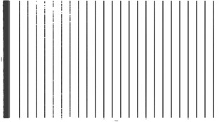
- What was I trying to do? I was trying to plot average colour versus hour i.e. 0-23!
- Why is it a mess? Because no two average colours are identical so you have 146475 values on the y axis which won’t fit on any display less than 146475 pixels high :-). Well not unless you have the world’s largest screen!
- Part 2 will explore changing the colours to the 600 or so R colours.