R faceted geom_density ggplot2 corrupted is a mess aka learning experience :-)

Pontifications

UPDATE: I think I figured it out. I need to remove n<=5 over each 1 hour period of the 24 hour period not over the entire 24 hour time period of the data set.
Not statistically valid :-) again :-) again :-)
I don’t like this version aesthetically, I envisioned 24 versions of the previous blog post aka y axis limited to 0.0012 for hour 0 but I tried to use 0.0012 and it didn’t look good.
I guess I need to look at a real density plot :-) somehow

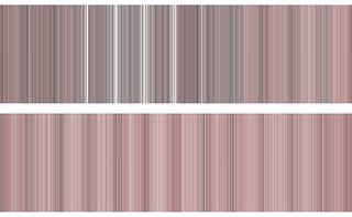
R ggplot2 geom_density() Code, no y axis limit, aes=colour (not the 600 R colours), faceted by hour, nrow = 2:

library(tidyverse)
library(plotrix)

getnumericColour <-
  function(colorname) {
    colour_matrix=col2rgb(colorname)
    return(as.numeric(colour_matrix[1,1]) * 65536 +
             as.numeric(colour_matrix[2,1]) * 256 +
             as.numeric(colour_matrix[3,1]))
  }
csv_url = 
"https://raw.githubusercontent.com/rtanglao/2016-r-rtgram/master/JANUARY2016/january2016-ig-van-avgcolour-id-mf-month-day-daynum-unixtime-hour-colourname.csv"

average_colour_ig_van_jan2016 = 
  read_csv(csv_url)

six_hundred_colour_ints_average_colour_ig_van_jan2016 <-
  average_colour_ig_van_jan2016 %>%
  add_count(colourname) %>%
  filter(n >5) %>%
  rowwise() %>%
  mutate(sixhundred_colourint =
    getnumericColour(colourname))
ggplot(
  six_hundred_colour_ints_average_colour_ig_van_jan2016, 
  aes(x=colour))+
  geom_density(mapping = aes(colour= colour_named_vector))+
  scale_colour_manual(values=colour_named_vector)+
  theme_void()+
  theme(legend.position = 'none') +
  theme(strip.background = element_blank(),
  strip.text.x = element_blank())+
  facet_wrap(~ hour, nrow = 2)

Pontifications

R ggplot2 geom_density() Code, no y axis limit, aes=colour (not the 600 R colours), faceted by hour, nrow = 2:

Output: